Milestone 1 Project - SIADS 591 & 592
February 3, 2021
Project Team:
Tim Chen (ttcchen@umich.edu), Sophie Deng (sophdeng@umich.edu), and Nicholas Miller (nmill@umich.edu)
Instructional Team:
Elle O'Brien (elleobri@umich.edu), Chris Teplovs (cteplovs@umich.edu), and Anthony Whyte (arwhyte@umich.edu)
GitHub Repository:
https://github.com/mads-hatters/SIADS-591-Orbital-Congestion
Space, and more specifically low-earth orbit, is about to get a whole lot busier and this is making many concerned. At present, there are about 2,000 operational satellites in low-earth orbit and more than double that in defunct satellites. But last year in October, SpaceX requested permission to launch 30,000 Starlink satellites into low-earth orbit. This is in addition to the 12,000 that already received approval. These satellites have already begun interrupting astronomical observations, creating light pollution and increasing collision risks in an environment where a collision could trigger a chain reaction which not only endangers current and future satellites but also human lives.
For our project, we will be looking into the present situation with satellite counts, ownership, purpose, and their corresponding orbits. We will use visualization techniques such as spatial density charts, gabbard diagrams, and animated time series charts to illustrate orbital congestion and highlight intersecting orbits that have the potential for collision. In addition to satellite data, we will explore debris in space. Using this data, we intend to investigate several questions and present an analysis that can be used for future work.
| Data Source 1 | Space-Track.org |
|---|---|
| Name | Satellite Catalog and ELSET data provided by the Combined Force Space Component Command's 18th Space Control Squadron |
| Size of Data | Almost 50,000 cataloged objects in space, their metadata, and multiple daily historical ELSET data. |
| Location | https://www.space-track.org/documentation#api |
| Format | CSV Two-Line Element (TLE) Orbit Mean-Elements Message (OMM) |
| Access Method | Direct download, API Access, or open source Libraries More details below. |
Space-Track.org contains a number of vaste historic and up-to-date datasets for satellite tracking that can be accessed via an API. The following Request Classes were used for this project:
| Request Class | Description |
|---|---|
gp |
The general perturbations (GP) class is an efficient listing of the newest SGP4 keplerian element set for each man-made earth-orbiting object tracked by the 18th Space Control Squadron |
gp_history |
Listing of ALL historical SGP4 keplerian element sets for each man-made earth-orbiting object by the 18th Space Control Squadron. |
satcat_debut |
Satellite Catalog Information with satellite catalog debut time |
| Further information can be found here: https://www.space-track.org/documentation#/api |
To access Space-Track.org data, login credentials are required. Free accounts are available here: https://www.space-track.org/auth/createAccount. With an account, the API can be accessed via an online query builder or via a python package such as spacetrack. Both of these methods were used for this project.
| Data Source 2 | Satellite Conjunctions Predictions (SOCRATES) |
|---|---|
| Name | Satellite Orbital Conjunction Reports Assessing Threatening Encounters in Space |
| Size of Data | Up to 1,000 entries of predicted satellite or debris conjunction entries for the next 7 days. |
| Location | https://celestrak.com/SOCRATES/ |
| Format | HTML |
| Access Method | Web scraping to CSV files |
SOCRATES calculates the likelihood two satellites will collide based on recent satellite location and orbit via TLE data. The website displays upto 1000 satellite pairs based on either maximum probability of collision, minimum distance between satellites or sorted time of closest approach.
| Data Source 3 | NTRS - NASA Technical Reports Server |
|---|---|
| Name | History of On-Orbit Satellite Fragmentations, 15th Edition |
| Size of Data | a document of size 3954 KB |
| Location | https://ntrs.nasa.gov/ |
| Format | |
| Access Method | Download from the server |
NASA provides a history of satellite break-ups which is useful in determining when debris from break-ups originated since Space-Track.org data only has the date the debris is first tracked.
SOCRATES is a web service provided to the satellite community by the Center for Space Standards & Innovation (CSSI) which provides information on pending intercepts of satellites within a week. This information is valuable for predicting if and when two satellites collide based on probability and estimated minimal distance.
To capture this information, a web scrapper called socrates_scrapper_nm.py was developed using the BeautifulSoup python package. The web data is tabularized and contains a single conjunction event across two rows which made using pandas built-in scrapper less reliable:
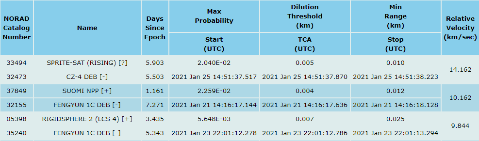
Twice a day, the information is updated and produces a massive amount of data, therefore, SOCRATES provides three different methods for retrieval [Maximum Probability, Minimum Range, Start Time]. And the maximum number of rows retrieved for each is 1000 events. Because of this, the web scrapper loops three times capturing the maximum amount of data.
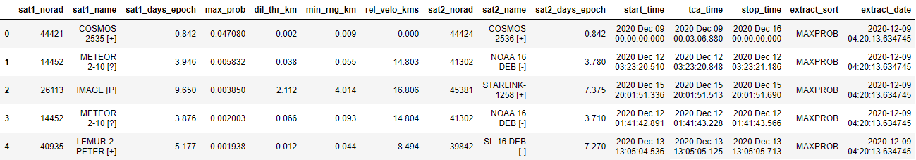
The scrapper was written to run as a background job with output messages sent to a log file. Each execution of the scrapping job dumps the results into a new dataframe which is then saved in ./data/socrates/socrates_YYYYMMDDHHMISS.csv.gz. The resulting structure:
One of the goals was to visualize the close encounters reported by SOCRATES in an effective way. To accomplish this, the TLE for each satellite is necessary. Getting the latest TLE for a satellite results in a large margin of error which is one of the reasons why TLEs are frequently updated. Space-Track.org has a retrieval class called gp_history for historical TLE records that was used for this data collection.
One of the challenges in accessing the historic TLE data is that the API used to retrieve gp_history data is limited to 300 requests per hour. While exceeding it is possible and was done initially, Space-Track.org sends an email warning that repeated violations result in a permanent ban. Since each SOCRATES grab resulted in 3000 satellite pairs twice a day, creativity was necessary to grab the data in larger chunks and thus limiting the number of requests. This was accomplished by looking at all the SOCRATES data and comparing that to the TLE data previously retrieved and getting a list of missing (new) satellite pairs. Each satellite then needed an epoch date—the date of when a TLE was captured—to know which TLE should be retrieved from gp_history. SOCRATES didn’t contain this date but instead contained a “Days Since Epoch” value allowing for the backdate calculation. This unfortunately had an error of about five minutes but TLEs are at most captured every 30 minutes and usually are hours or days apart for one satellite.
To address the soft cap of 300 requests an hour, the missing data was sorted by epoch date and grouped in batches of approximately 100 and assigned a bin number. Each bin would represent a single request. The request was then built passing a list of satellite NORAD ID numbers that existed in the batch and a start/end epoch window. This could result in the API returning multiple TLEs for the same satellite so the results needed to compare the epoch on the TLE to the approximate epoch calculated previously. The captured TLEs were saved off to a CSV as a safe guard if the merging process should fail so another API grab wouldn’t be necessary (this redundancy was never needed). The merging process consolidated each satellite pair with their TCA (time of closest approach) and appended the data to the TLE grab dataframe which would later be joined on demand with the SOCRATES data.
The code for this TLE grab and merging takes place in a script called socrates_gp_history_tle_grab_nm.py. This script was executed after each run of the web scrapper via a background job on a personal computer left on for about two months.
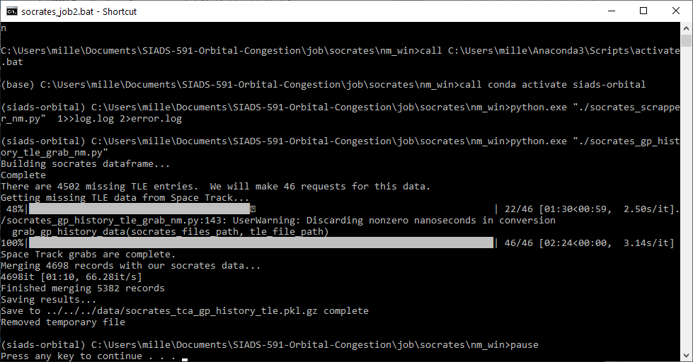
Above is an example manual run. The first stage is the web scrapper which sends the output to a log file log.log. The second stage is the TLE grab shows the grab of 4502 missing TLE entries grouped into 46 API requests and then after merged with the SOCRATES TCA for each pair.
Since the raw SOCRATES data contains many duplicates, there might be cases where the raw data might be analyzed and other cases where only the unique records joined with TLE entries would be necessary. To resolve this challenge, a new python package socrates was created with several different options for loading the SOCRATES data. Those functions include:
get_all_socrates_data() - This loads only the raw SOCRATES data from all available files and merging them together without any cleaning of duplicate records.get_socrates_cleaned_data() - This calls get_all_socrates_data(path) and drops duplicates, keeping only the most recent.get_socrates_with_tle_data() - This merges the SOCRATES dataset (e.g. from get_socrates_cleaned_data()) with the TLE data grabbed for SOCRATES.get_all_socrates_and_tle_data() - This calls get_socrates_cleaned_data() and get_socrates_with_tle_data() and returns two datasets: the cleaned SOCRATES data and the merged data.One issue with the data from Space-Track.org is the origin date of debris resulting from the breakup of satellites is the date the debris is first tracked and not the date of the satellite breakup. Tracking the date of breakup events is crucial to analyze the number of debris available over time as it provides accurate information on when debris were created and subsequently decayed. This information can be found in the form of tables from a PDF report called "History of On-Orbit Satellite Fragmentations" from NASA.
To extract table information from the PDF, a library named Tabula was used:
Install and set up Tabula (windows): Pip install tabula-py and java. If there’s a FileNotFoundError when it calls read_pdf(), set PATH environment variable to point to the Java directory.
The challenge of using Tabula comes from not reading the tables in PDF file according to the original page breaks. Tabula breaks 8 tables in 8 different pages into 20 dataframes which need to be manually cleaned and combined. In other words, if the satellite name spans multiple rows, Tabula splits it incorrectly into two rows, resulting in a second row with NaNs. Manual cleaning also involves update date format not recognized (i.e. 3/4Aug-15, ~21-Dec-11), removing footnotes and unnamed columns.
CesiumJS is an open-source GPL library that looks similar to the popular Google Earth platform. It is highly customizable and allows for painting of custom shapes and images onto and around a 3D model of the Earth built from satellite imagery. Since the imagery is licensed, a free API key is necessary to create the visuals.
Getting Cesium to display properly on the Plotly Dash dashboard turned out to be challenging due to how Dash creates the different objects and calls javascript methods. After asking on Plotly Dash community pages and stackeoverflow, help was received on how to get around this problem.
The Cesium platform also supports a file format called CZML, used to create time-based animations. To take advantage of this, the python package tle2czml, developed by Shane Carty, was initially used to animate the intercepts of two satellites on the dashboard. However, this package is quite limited in functionality. For example, the coloring, markers, and marker descriptions are all static. An improvement to allow custom descriptions was made and a pull request was initialized but the developer hasn’t responded at the time of this writing. Because of these limitations, a custom python library called satellite_czml was created, which is now available as a python package available on PyPI.org and is open source on GitHub. The packge can be installed by calling the following:
pip install satellite-czml
This python package, like tle2czml, relies on a custom version of another python package called czml, developed by Christian Ledermann and the python package sgp4, developed by Brandon Rhodes (coincidently, the same developer of skyfield, discussed below). satellite_czml is now used in the dashboard to create the intercept and Starlink animations.
Space-Track provides a gp_history API for accessing all historical satellite TLE data. For the initial exploration and static charts, individual CSV files from the gp_history request class (request classes documentation) generated by the query builder was manually downloaded. However, this process was tedious and did not scale when comparing multiple satellites across different time periods, which is necessary for maneuver detection. Also considering other analysis which rely on gp_history, an automated processes to acquire bulk data became a necessity.
Some challenges that had to be resolved for bulk downloads
| Challenge | Description and resolution |
|---|---|
| API limitations | The API has a hard limit of 100,000 entries per request and a rate limit of 30/minute and 300/hour. With the gp_history data sitting at nearly 150 million entries, under optimal situations, 1,500 API calls over a period of 5 hours at the minimum. |
| API authentication | The API requires authentication using individual username and password. Credentials template files needed to be shared while individual crential files needed to be excluded from source control. |
| Authorization duration | The API only offers access tokens with 2 hour lifetime, with the large amount of long running jobs, resuability and automaticated re-authenticate was necessary. |
| Platform support | An ideal long term solution should be cross-platform as the team's development machines consisted of Windows and Mac. A method to have a jupyter notebook automatically run code was developed to avoid platform specific schedulers or a separate backend (see skeleton_autorun_below.ipynb for proof of concept and skeleton code). |
| Keeping data up to date | The process must allow incremental updates when new data becomes available while ensuring that no entries are missed. |
Initially, the script only downloaded satellite data with various LEO configurations in chronological order, however, sometimes data entries will be missing or spike when specific parameters cross certain thresholds (e.g. the LEO requirements). Ultimately, the script was modified to download practically all of the data with local filtering being performed based on specific data needs at a later time. The current numbers as of Jan 26th, 2021: 144,800,000+ gp_history entries stored in 1,449 files, taking up 80GB storage. These raw files are then compressed and stored without further processing as different analysis may require different columns.
The code for this download process can be found at download_all_gp_history.ipynb.
Maneuver detection is possible by looking at abnormal readings in the TLE data. Initial exploration was done visually using data segments downloaded manually from Space-Track. Maneuvers are generally easy to spot visually, however, with the large amount of data, manual inspection for maneuvers could not scale. Automatic maneuver detection was needed. This section will provide an overview of how the data is pre-processed. Maneuver detection methods will be discussed in the analysis section.
| Challenge | Description |
|---|---|
| Data Frequency | Interval between TLE entries varies a lot - from 1 entry in 3 months to less than 2 hours between 2 TLEs. Some normalization is needed when using .diff() to examine the data. |
| Data Accuracy | Some data contains obvious errors which may be due to sensor errors or attributing TLE data to the wrong entity. There are also some duplicates in data that affects rolling windows using .rolling() and using .diff() to look at changes in data. |
| Memory Requirements | Due to the size of the data, loading in all the data has a really high memory demand. |
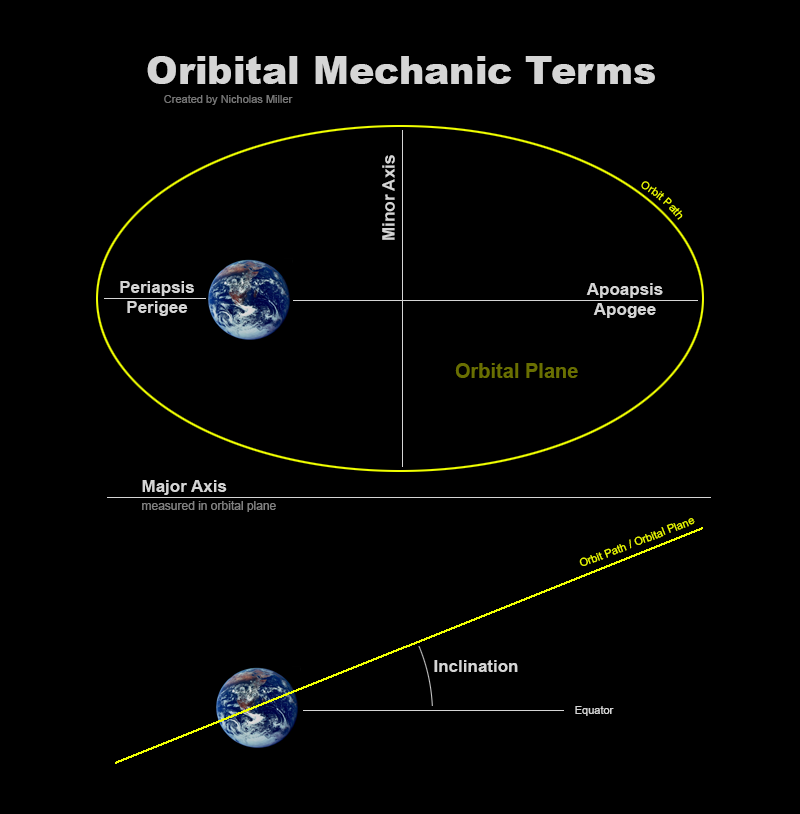
When examining ISS's orbit data, some of the orbital elements appear to have direct correlation (such as MEAN_MOTION, SEMIMAJOR_AXIS, PERIOD, APOAPSIS, and PERIAPSIS, as well as BSTAR and MEAN_MOTION_DOT) while others are less suitable due to their periodic variance and noise (such as ECCENTRICITY, ARG_OF_PERICENTER, and MEAN_ANOMALY).
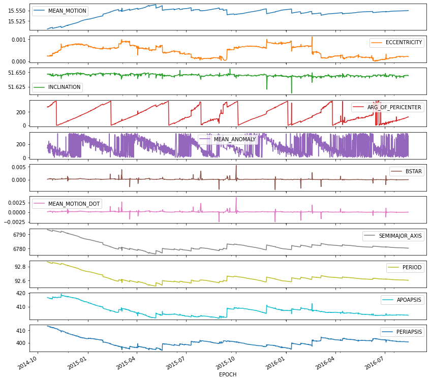
Further research (NASA - Satellite Safety) revealed that satellites mainly maneuver by raising or lowering their orbits, or adjusting their inclination. A decision to only look at SEMIMAJOR_AXIS and INCLINATION to determine orbital maneuvers was made. This resulted in a reduction of 9 columns from the dataset.
dtype Conversion¶However, with over 32,147,425 rows of TLE data for the artficial satellites, it still took up significant memory and further reduction was preferred. With the data being stored as 64-bit numbers, the use of 16 and 32-bit numbers were considered.
| Column | Import dtype |
Notes | Final dtype conversion |
|---|---|---|---|
| EPOCH | object |
While another data type instead of datetime64 could have been used to represent a time component, a decision was made against it due to the loss of convenience when slicing data by time. Also of note that a 32bit representation would likely lead to the smallest time step in seconds, which could potentially be a problem when exploring maneuver some collision predictions put satellites in the same block of space with in milliseconds of each other. |
datetime64 |
| NORAD_CAT_ID | int64 |
A NORAD ID is assigned to each piece of space object. Currently, artificial satellites have NORAD IDs up to the 47,000 NORAD IDs range, making the unsigned 16-bit integer uint16 a perfect choice for the near term*. |
uint16 |
| INCLINATION | float64 |
Inclination has a value range of 0-180. Initially, float32 was considered for an easy conversion, however it introduced precision loss. Since Space-Track provides the data with a maximum of 5 decimal point precision, the number was stored as uint32 after multiplying it by 10,000. |
uint32 With 10,000x scaling |
| SEMIMAJOR_AXIS | float64 |
Semimajor Axis received a similar treatment to Inclination, but with a 1,000x scale instead due to its 4 decimal point precision. | uint32 With 1,000x scaling |
Note : While uint16 should be sufficient to represent NORAD_CAT_ID for the current data, it is important to keep in mind that 80,000-89,999 range is assigned to objects with insufficient fidelity for publication in the public satellite catalog (Space-Track FAQ), and that the SATCAT is growing at a much quicker rate compared to before. The Combined Force Space Component Command also has increased tracking capacity with the introduction of a new Space Fence on Kwajalein Atoll in March 2020. With over 200 objects being added to the SATCAT in Jan, 2021 already, the maximum allowable value for uint16 of 65535 may be reached rather soon (currently at 47,436 as of writing).*
Here are the final reduction results from a sampled slice from the entire dataset (results can be found at filter_raw_data_payload_maneuvers_report_data.ipynb):
| Processing Stage | Number of Entries | Number of Columns | Column dtypes |
DataFrame Memory Usage |
|---|---|---|---|---|
| Raw CSV Input | 100,000 | 40 | float64(14)int64(6)object(20) |
30.5+ MB |
| Filtering LEO artificial satellites | 23,126 | 40 | float64(14)int64(6)object(20) |
7.2+ MB |
| Remove non-Orbital Element columns | 23,126 | 16 | float64(13)int64(2)object(1) |
3.0+ MB |
Reduce Orbital Element columns to SEMIMAJOR_AXIS and INCLINATION |
23,126 | 4 | float64(2)int64(1)object(1) |
903.4+ KB |
dtype conversion |
23,126 | 4 | datetime64[ns](1)uint16(1)uint32(2) |
406.6 KB |
| Full maneuver dataset with conversion | 32,147,425 | 4 | datetime64[ns](1)uint16(1)uint32(2) |
551.8 MB |
The code for this reduction process can be found at filter_raw_data_payload_maneuvers.ipynb.
With the increasing amount of satellites in Low Earth Orbit, an increased frequency of risk mitigation maneuvers is expected. To verify this hypothesis, data from the CelesTrak's SOCRATES dataset was again used. SOCRATES uses the same TLE data available from Space-Track to calculate potential satellite conjunctions for a 7 day period. With the SOCRATES data, pairs of satellites on a collision course (can be visualized in the dashboard) were identified, however, the information is limited to a specific time. In order to detect maneuver, a series of TLE data surrounding the conjunction time is required. Grouping of the predictions made was also needed to determine how the collision probability has changed during that 7 day period for each incident.
To get the SOCRATES history of a particular possible collision, all the SOCRATES reports where combined into one DataFrame then grouped together based on the satellite pairing and the Time of Closest Approach (tca_time). Additional data manipulation was needed to set the proper group for tca_time due to pairs of satellites having multiple conjunction events. To filter down the selection further, entries which only contain objects that are known to have no maneuvering abilities, such as debris or spent rocket bodies, were removed. Non-LEO objects were also elimited as they were out of scope of the project. Finally, events with a predicted max_prob of 0.5% or greater were selected to do further investigations.
With the maneuver dataset process already completed in the previous section, applying the appropriate NORAD_CAT_ID and EPOCH time range filter was the only necessary step to obtain the satellite data. A time range of 14 days prior to the first time a conjunction event was predicted to 5 days after the tca_time was chosen to provide the maneuver detection algorithm plenty of data to find maneuvers and to provide context during visual inspection of the individual events.
The satellite catalog (SATCAT) was also merged to provide names of the satellites since some of that information was removed from an earlier reduction process.
The code for this pre-processing can be found at detect_maneuver_from_socrates_suggestions.ipynb.
A Gabbard diagram shows the PERIOD of objects on the x-axis and their APOAPSIS and PERIAPSIS on the y-axis. An animated version of the Gabbard diagram would need these data over a period of time.
Proof of concept for the animation was done using a small timeframe by grouping entries using the dt.week. This was not an ideal solution though, because week numbers do not reset with a year change, resulting in a flashback frame every year, and none of the aggregate features represented the satelite's position well due to how wide the time window was.
Since a datetime groupby cannot be used, reindex and interpolate were used instead to have a more accurate representation of the data. A proof of concept was done by first performing a unstack so each satellite has its own column, then performing a reindex over the entire time period and interpolate missing data in between. However, this failed to scale spectacularly as the DataFrame size is now m n where m is the number of objects 3 (one for each of PERIOD, APOAPSIS, and PERIAPSIS) and n is the number of frames - exceeding billions of cells.
An alternate strategy was developed, where each satellite would only generate its own valid time range in order to avoid the NaN cells prior to the it being tracked or after it decayed. This was achieved by performing the split-apply-combine process, grouping by NORAD_CAT_ID then applying the datetime index transformation along with the interpolation. Due to some errors in the data in the late 1970s, where incorrect TLEs were being attributed to satellites, it was also necessary to remove some outliers and to not interpolate impossible cases.
dtype Conversion¶To reduce memory usage, dtype conversion similar to the earlier maneuver detection process was applied. However, there is a difference in that the data for Gabbard diagrams allow for some precision loss since it can hardly be noticed due to the limited size of the charting area. This allows additional optimization when looking for a suitable dtype to use. The dtype conversion will be applied prior to grouping and interpolation. Every little bit (Ba Dum Tss!) counts with the with 86,326,993 rows of data!
| Column | Import dtype |
Notes | Final dtype conversion |
|---|---|---|---|
| EPOCH | object |
Since further time-based grouping will be done at a later step, the datetime64 precision was preserved for sanity purpose. |
datetime64 |
| NORAD_CAT_ID | int64 |
Similar to the earlier conversions, the NORAD_CAT_ID can be represented as an unsigned 16-bit integer for the near term. |
uint16 |
| APOAPSIS | float64 |
For the purpose of generating LEO Gabbard diagrams, an APOAPSIS of > 3000 is out of range, thus, APOAPSIS can be represented by a uint16 after a 20x scale resulting in a max precision of 1/20 step |
uint16 With 20x scaling |
| PERIAPSIS | float64 |
Similar to APOAPSIS, the same conversion can be applied to PERIAPSIS for a max precision of 1/20 step |
uint16 With 20x scaling |
| PERIOD | float64 |
The orbital PERIOD for LEO Gabbard diagram does not exceed 130 and can be scaled by 500x for nearly no precision loss (1/500 step vs 1/1000). |
uint16 With 500x scaling |
*Note: pd.UInt16Dtype() will both be used for the pd.NA support for integers which will come into play during the reindexing step prior to interpolation. However, Pandas Integer types are not supported by pd.DataFrame.interpolate() and np.uint16 will be used during the interpolation step.
The code for pre-processing this data can be found here: filter_raw_data_gabbard.ipynb and the reindex and interpolation code can be found at: process_gabbard_data_interpolated.ipynb.
To annotate events in the animated gabbard diagram, data from the Satellite Breakup PDF section was used. Initially, all the data was filtered automatically based on time and orbit, however, manual selection was needed due to the clutter of many minor events during certain years, as well as some data being nearly invisible in the diagram. In the end, 79 events were chosen for their prominence and magnitude. One event was added (2019 Microsat-R anti-satellite test) as it happened after the publish date of the document, and another required manual attribution for debris pieces due to that particular launch being related to two multiple events (all other breakup events came from different launches).
The code for generating the gabbard diagram animation can be found at animated_gabbard.ipynb and the manually updated and annotated breakup file is stored as breakup_custom.csv.
A dashboard was created to summarize and present, in an accessible way, some of the interactive visuals discussed in this report. The dashboard can be accessed either online via Heroku or by running the notebook oc_dash.ipynb in the source. Both options use the same source code and data sources.
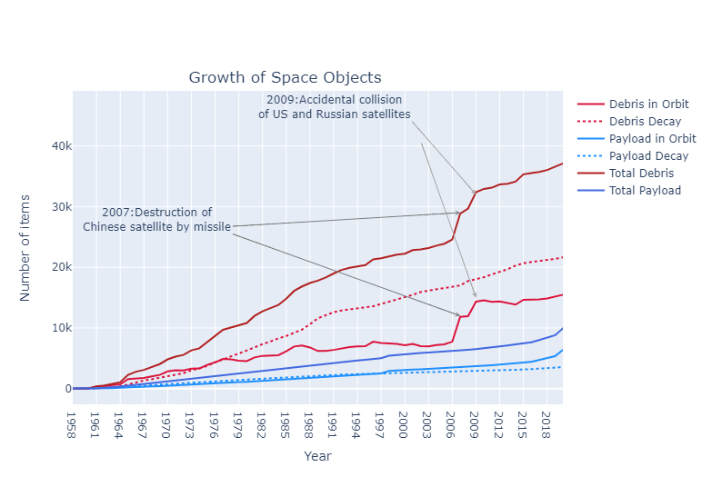
In the past 60 years, the space around the Earth has gone from a virtually debris-free environment to a zone cluttered with man-made objects that potentially threaten launches, active satellites, and the International Space Station (ISS). Below time series graph illustrate the historical growth of space debris including rocket body as well as payload (i.e. satellite and spacecraft).
The amount of debris in orbit has been increasing since 1958. The rate of growth slowed for a decade from 1996. However, the destruction of the Fengyun-1C weather satellite in 2007 and the collision of the inactive Russian satellite Cosmos and the active U.S.-based communication satellite Iridium in 2009 reversed that trend, creating at least 4000 pieces of debris. As a result, it increased the risk of impacts to the ISS by an estimated 44 percent over a 10-day period. (Wei-Haas, 2019).
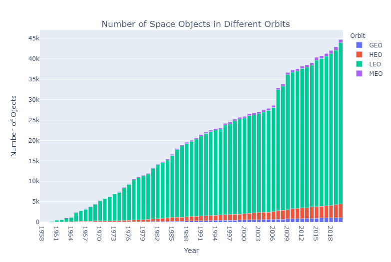
In addition to above time series analysis, the bar chart below provides another view on the number of space objects in different orbits. Evidently, low-earth orbit (LEO) has the highest object count among all orbits stated. In 2020, approximately 80% of space objects are in LEO. LEO has become an orbital space junk yard. According to NASA, most “space junk” can reach a speed of 18,000 miles per hour, almost seven times faster than a bullet (NASA, ret. 2020). Due to the rate of speed and the increasing number of debris in LEO, current and future space-based activities pose a safety risk to people and property in space and on Earth. The problem of managing space debris is every spacefaring country's responsibility and immediate action is needed to preserve the space environment.
An issue with evaluating the congestion of space is that satellites are not evenly spaced around Earth but rather are concentrated in different orbital bands (altitudes). These congested orbits are where risks of collision are greatest. Here is an animation that illustrates how this congestion has changed over time.
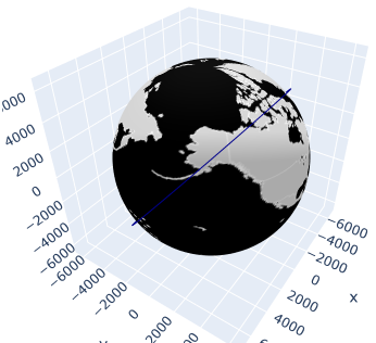
To effectively visualize the orbits and intercepts of satellites, several options for presenting 3D visuals were researched. Matplotlib and Plotly both provide 3D plotting functionality and are common libraries used in Python, although, matplotlib lacks the interactivity necessary to navigate a satellite orbit. Because of this Plotly was first utilized.
Plotly does have the capability for painting an image onto a 3D surface but only one color channel can be applied. Also, since Plotly is utilizing functionality not designed to paint 3D surfaces with images, the image resolution must be kept at a minimum to improve performance. In the end, a black and white, stereographic image of the earth was used to create an earth-like sphere. To place a satellite marker on the Plotly 3D image, the Python package skyfield was used which offers the EarthSatellite() convenience function and outputs an x,y,z coordinate in kilometers with the center of the earth as the origin.
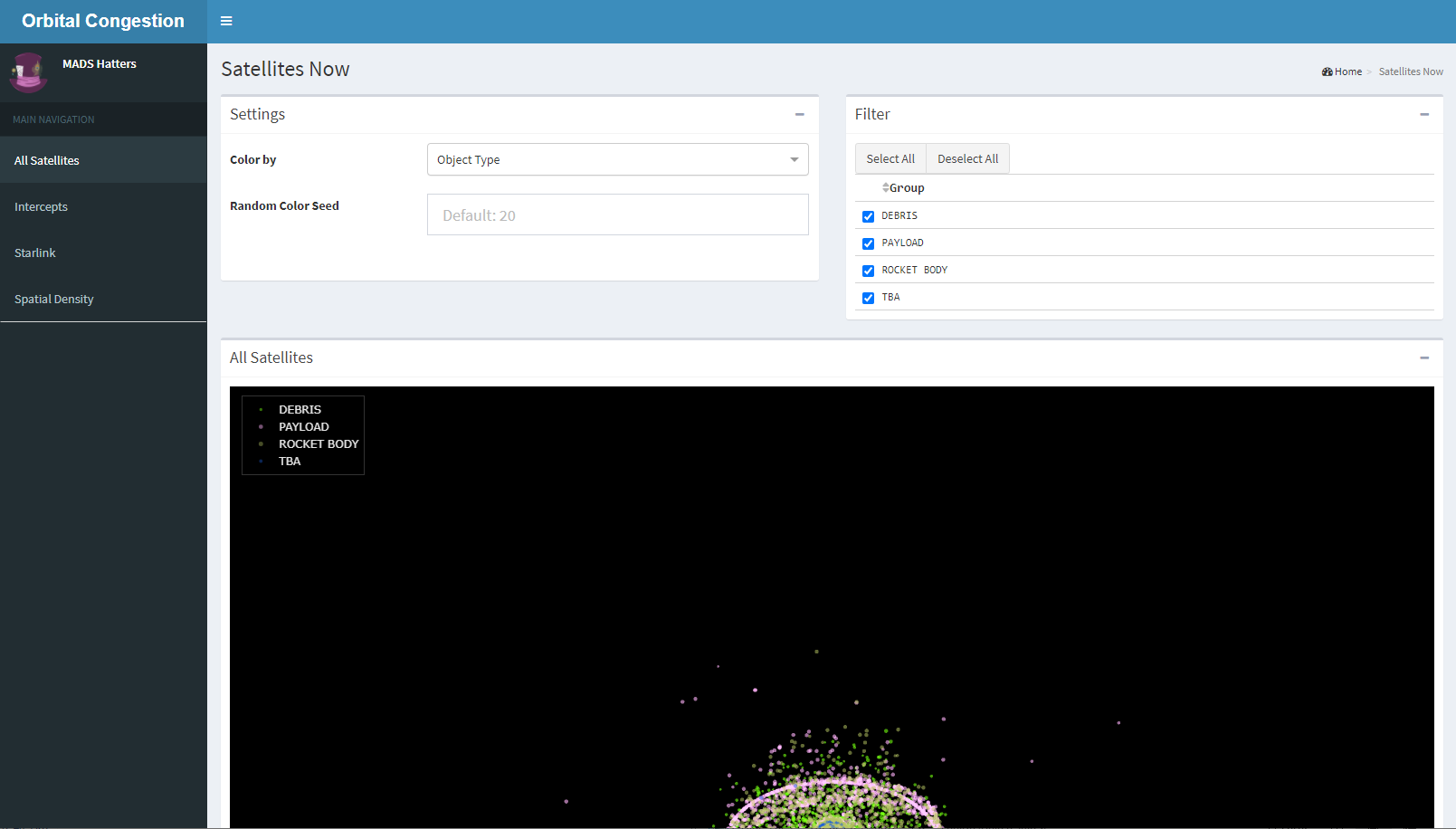
One of the goals for the dashboard and the reason for creating the satellite_czml python package was to visualize all the satellites in orbit on the present day using Cesium. However, after assembling the pipeline to build and display the satellites, the amount of data proved to be too much and the visual was never able to load. The amount of data necessary to plot over 20,000 satellites using a CZML string was slow and the amount of data too large for a timely response. Using Javascript methods to calculate position instead of using CZML would have likely been a more suitable approach but this was abandoned due to time restraints in favor of using a 3D Plotly visual. Joined with Dash, the visual allows for the user to specify color coding and filtering options and the interactivity includes details for each satellite on mouse-hover.
With the creation of satellite_czml package with Cesium, plots for intercepts and Starlink satellites reflect accurate satellite position, time of day and motion in an interactive environment. Each satellite also contains a detailed description with a dynamic hyperlink to more information about a selected satellite. These visualizations illustrate the congested and variations in near-collisions that are at risk of occuring daily.
The ability to detect whether a satellite performed a maneuver is needed in order to perform analysis on whether a satellite performed a risk mitigation maneuver (RMM) or not. Artificial satellites with propulsion can adjust their orbit by performing two types of maneuvers. The first is a orbit raising/lowering maneuver, where orbit raising is normally performed to counter the effects of atmosphere drag or to avoid other satellites. Orbit lowering maneuvers are sometimes performed by braking instead during RMMs if an orbit raising maneuver is not an option. The second type of maneuver is an inclination adjustment maneuver where the inclination is adjusted to keep the orbit within certain parameters (NASA - Satellite Safety, ret. 2021). Semimajor axis and inclination metrics of eight selected satellites will be examined to see if maneuvers can be detected correctly. For simplicity, data will be examined in isolation from each other.
| Selected Satellite | NORAD ID | Time Range |
Reason | |
|---|---|---|---|---|
| AQUA | 27424 | 2008/10 to 2010/10 | From visual examination, AQUA performed multiple orbit raising and inclination adjustment maneuvers during this time frame, making it a good candidate. | |
| OCO-2 | 40059 | 2017/12 to 2018/05 | OCO-2 also performed multiple orbit raising and inclination maneuvers in the selected period while showing little to no noise in the metrics. | |
| Fermi Gamma-ray Space Telescope (GLAST) | 33053 | 2011/12 to 2012/10 | NASA revealed that GLAST performed an evasive maneuver in April of 2012. It had not performed any other maneuvers prior to this since being put in orbit (NASA | Fermi's Close Call with a Soviet Satellite, ret. 2021</a>). |
| International Space Station (ZARYA) | 25544 | 2020/01 to 2021/01 | The ISS is the largest artificial object in space and performs many maneuvers to raise its orbit and had to maneuver to avoid other objects previously, making it an interesting satellite to look at. | |
| GCOM W1 | 38337 | 2016/03 to 2017/09 | NASA documented 5 RMMs during the indicated time range. They are relatively spaced out and should be distinctly identifiable. | |
| COSMOS 2251 | 22675 | 1993/06 to 2021/01 | The COSMOS 2251 actually do not have a propulsion system, however, its orbit did change due to its collision with IRIDIUM-33 in 2009. Examining it's entire life span will also allows for the evaluation of the maneuver detection method over a long period of time. | |
| PAYLOAD C (Shiyan 7) | 39210 | 2013/08 to 2019/01 | PAYLOAD C, or Shiyan 7 (SY-7, Experiment 7) is a Chinese satellite that possesses the ability to greatly alter its orbit rapidly, it made a series of big maneuvers in its first 3 years of service and continued to make tiny adjustments after that (SPACEPOLICYONLINE.COM | Surprise Chinese Satellite Maneuvers Mystify Western Experts, ret. 2021</a>). |
| STARLINK-1007 | 44713 | 2019/11 to 2021/01 | A Starlink was included due to SpaceX being one of the main contributors for recent increase in Low Earth Orbit satellites. STARLINK-1007 is amongst the first operational Block v1.0 Starlinks that were launched. |
Various methods and thresholds for detecting maneuvers were examined for their effectiveness. For each satellite, multiple exploratory charts were generated for visual evaluation.
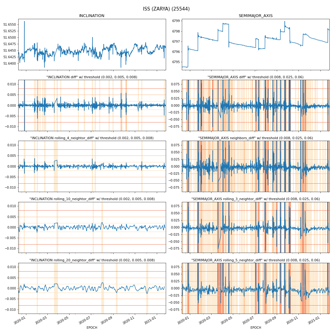
The above chart explores potential maneuver detection methods based on ISS data - lots of potential orbit raising and lowering maneuvers were detected, likely being overly sensitive, while showing almost nothing on inclination adjustments. Similar charts for the other satellites are availble to view on the dashboard or can be found at images/maneuver_analysis.
In the above chart, the left set of images represents detection methods for inclination adjustment maneuvers, while the right column represents detection for orbital raising / lowering maneuvers. These detection methods are ordered by sensitivy, with the diff type detection being highly sensitive while a large rolling window being less sensitive. Multiple thresholds were also selected for each method. The resulting graphs highlight time ranges in orange where maneuvers were detected. The lighter orange shades are detected by the most sensitive thresholds and while the darker orange shades only show more obvious maneuvers.
Based on the results, rolling_10_neighbor_diff, comparing two rolling windows with size of before and after a point, with a threshold of 0.008 was selected for detecting inclination adjustment maneuvers, and a rolling_3_neighbor_diff with a threshold of 0.025 was selected for detecting orbit raising / lowering maneuvers. The results:
Satellite |
Note | Resulting Image |
|---|---|---|
| AQUA | Detected most of the maneuvers, however 3 were missed in early 2010. | 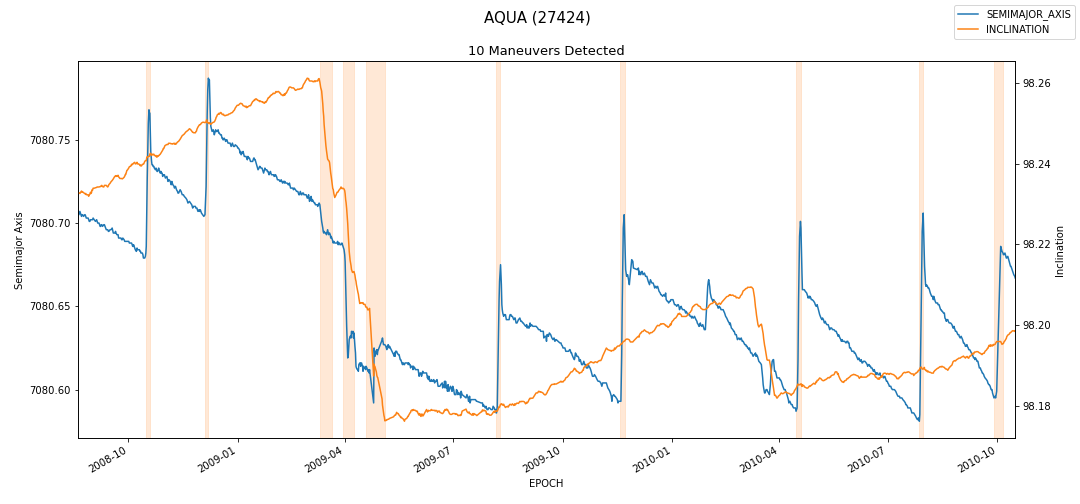 |
| OCO-2 | Successfully detected all maneuvers. | 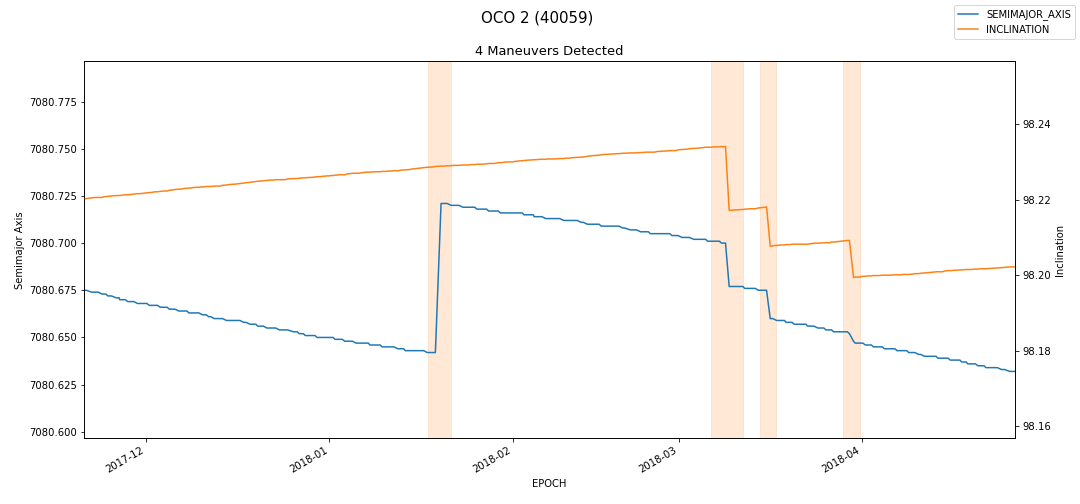 |
| Fermi Gamma-ray Space Telescope (GLAST) | Detected the RMM, but also falsely identified 5 other maneuvers. | 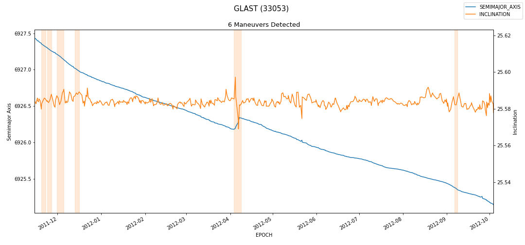 |
| International Space Station (ZARYA) | Ground truth maneuvering data for ISS maneuvers is unavailable, however, it looks like the major maneuvers were picked up, with a few potential false positives. | 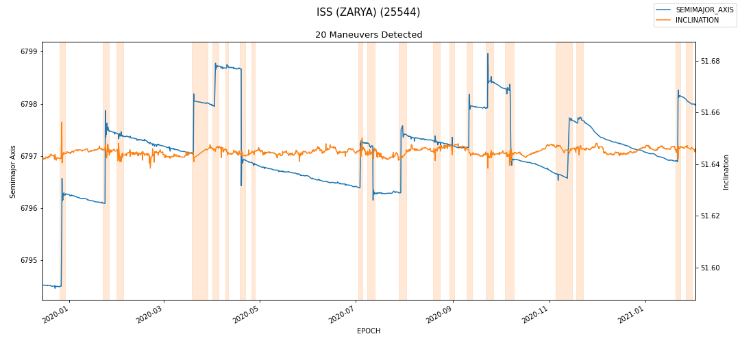 |
| GCOM W1 | Ground truth data is also not completely available, however the 2017/05/30 RMM failed to detect successfully. | 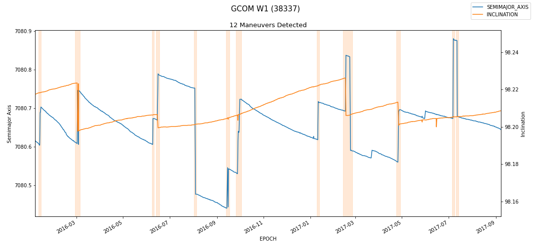 |
| COSMOS 2251 | The collision with Iridium-33 was positively identified, however there were also two false positives, likely due to error in the data. | 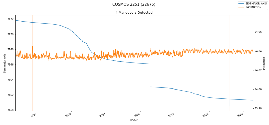 |
| PAYLOAD C (SY 7) | Shiyan 7's big maneuvers were all identified, however, other candidates were inconclusive because of the lack of ground truth data. | 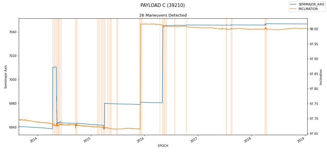 |
| STARLINK-1007 | Starlinks were detected as being constantly maneuvering. After cross-checking this with other Starlinks, it would appear that unlike other satellites where they would allow their orbit to decay and do occasional adjustments, Starlinks actually are constantly re-adjusting their orbits to maintain very specific operational parameters. | 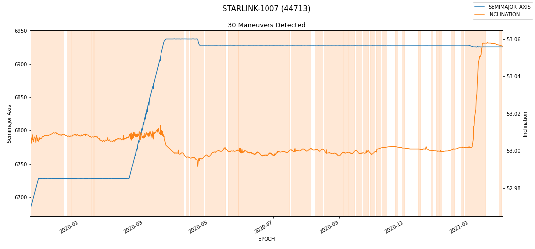 |
The code for generating the combined detection and different detection methods with thresholds images can be found at maneuvers_detection_method.ipynb.
While this could definitely be improved by taking into account other factors such as specific operational parameters (like Starlink's), solar activity, inclination variance, and orbital decay based on altitude, with this combination of detection methods and thresholds, the majority of the maneuvers has been identified and should be sufficient for identifying RMMs.
Collisions between objects in space are hypervelocity collisions where the velocity (v) of the impactor (relative to the target) is so great that its kinetic energy ( $K = \frac{m v^2}{2}$) is greater than the energy released in the detonation of the same mass (m) of high explosive. (Australian Space Academy, ret. 2020)
In low Earth orbit, the velocity of a satellite is between 7 and 8 km/sec and the typical collision velocity between two space objects in LEO is around 10 km/sec. An accidental LEO collision will most likely be a hypervelocity collision. The deliberate destruction of a satellite with a launched missile is also a hypervelocity collision. A hypervelocity collision may be categorised as catastrophic or non-catastrophic. A catastrophic impact results in both the target and the impactor being totally destroyed while in a non-catastrophic event, the impactor is detroyed and the target is damaged.
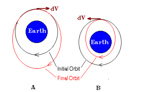
Fragments ejected from a collision will have a new orbit dependent upon the magnitude of the ejection velocity and the direction of this velocity vector with respect to the velocity vector of the satellite at the time of collision. If the velocity is in the same direction as the original target motion (A), the initial orbit will be turned into a larger elliptial orbit. On the other hand, if the velocity is in the opposite direction (B), the final orbit will become smaller than the initial orbit. This is illustrated in the figure below:
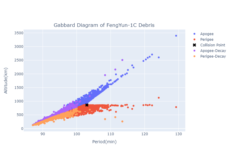
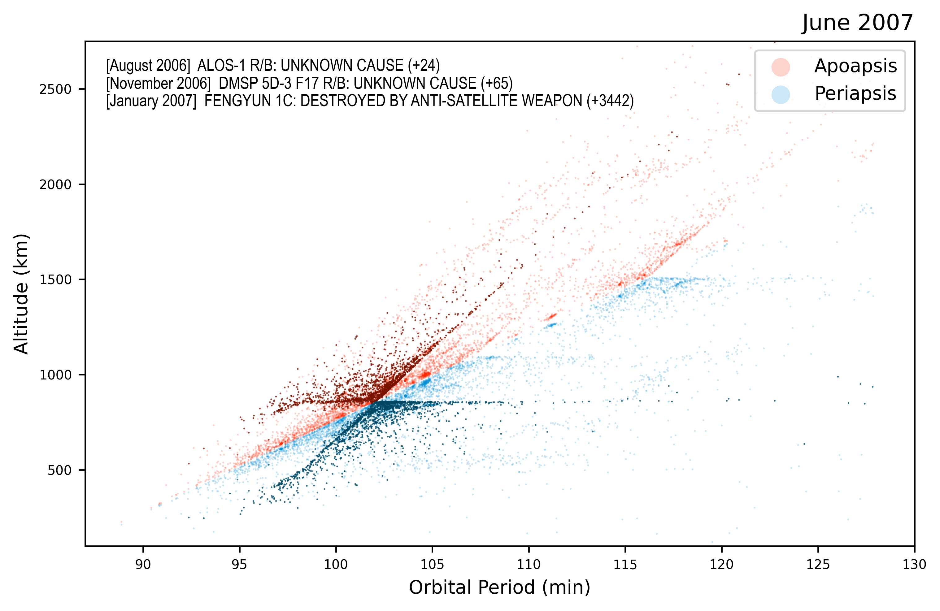
John Gabbard developed a diagram for illustrating the orbital changes and the orbital decay of debris fragments. A Gabbard diagram is a scatter plot of orbit altitude versus orbital period. Since all orbits are elliptical, a Gabbard diagram plots two points for each satellite: the apogee and perigee. Each pair of points will share the same orbital period and thus will be vertically aligned.
On 11 January 2007, a non-operational Chinese weather satellite, the Fengyun-1C (FY-1C) was destroyed by a kinetic kill vehicle (missle) traveling with a speed of 8 km/s in the opposite direction at an altitude of 863 km.
The below Gabbard diagram illustrates the aftermath of this collision: 1) 3526 pieces of debris of trackable sizes are documented and 646 pieces have decayed.
2) The cross sign (x) marks the location of collision at the altitude of 863km which is low earth orbit(LEO). When a collision happens at a low altitude, some of the fragments ejected in the opposite direction to the original motion will be forced into orbits with a perigee below the Earth's surface. As a result, these fragments with smaller mass will generally burn up during reentry. Those of a larger mass tend to decay later due to their momentum until atmospheric drag causes them to deorbit.
3) Fragments with a perigee of less than about 100 km will encounter so much air resistance that they will never make it back to apogee, and will deorbit in less than one period. This explains the decay objects on the bottom left of the graph (purple and orange points) and the progessive drop in apogee as the period gets smaller.
On 10 February 2009, the Iridium 33 satellite collided with Kosmos-2251 causing massive debris clouds to form. To see if Cesium could be used to visualize this impact, the TLE data was gathered for the satellites just prior and after the collision. The resulting simulation successfully showed the two satellites paths intersecting in the artic circle.
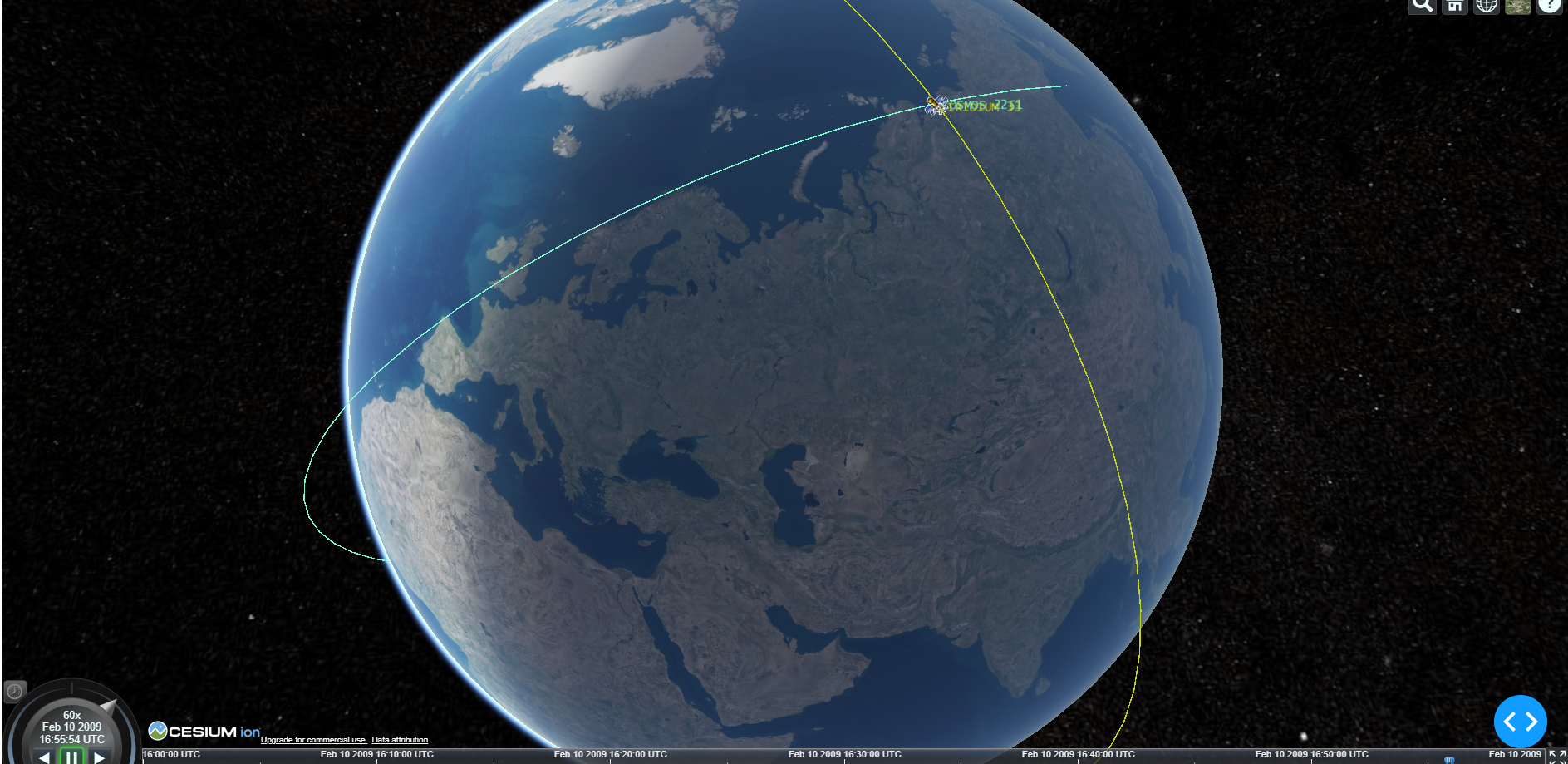
Next, the TLE data for each piece of debris was collected. Knowing that the TLE data for each piece of debris was collected after the collision, in some cases months after the collision, the debris position needed to be back dated to the time of the collision which would undoutably contain some error. After calculating the debris position at the time of collision using the first available TLE, Cesium showed debris scattered along each orbit instead of centered on the point of collision. The true error in the TLE data was overwhelming to the point that this exercise was scrapped.
To visualize the high probability collision predictions from SOCRATES, Cesium was used and animated to allow for a realistic inspection of the point in time when two satellites nearly intercept. This visualization technique is web-based and supported within the dashboard. Through these visualizations, it becomes evident how minor changes in orbit will have major impacts on collision probability.
With the SOCRATES dataset and the maneuver detection function in place, it is now possible to examine whether any RMMs had taken place. 131 incidents where a predicted collision chance of greater than 0.5% were found according to SOCRATES, and maneuver detection for each incident was performed.
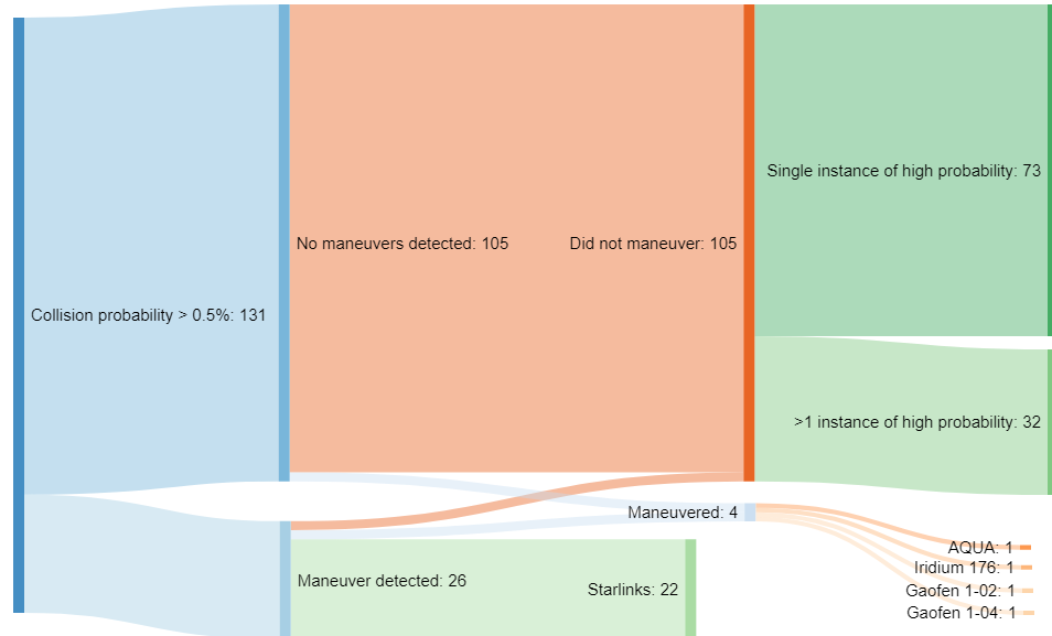
The following images show each satellite's semimajor axis, inclination, and detected maneuvers in the top chart while the bottom one shows the first relevant SOCRATES date in green, collision probability in purple, and the time of closest approach in red. The grey line represents when a new TLE entry became available, updating the satellites trajectory and position. In the case of a RMM happening, a maneuver period should be highlighted near or after the high probability being predicted.
Risk Mitigation Maneuver Group |
Description | Image |
|---|---|---|
| Starlinks | As shown in the maneuver detection part, Starlinks are constantly changing their orbits to maintain their operational parameters and it's difficult to judge whether they performed an RMM or not. Due to their constantly adjusting orbit, SOCRATES predictions are almost meaningless. | 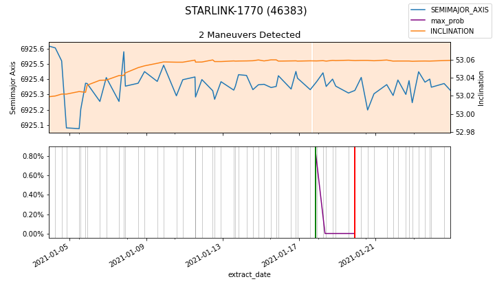 |
| AQUA | AQUA performed a maneuver that the maneuver detection missed, however, the maneuver was made outside of the SOCRATES prediction window. AQUA did not maneuver after SOCRATES predicted the 0.582% conjunction chance. | 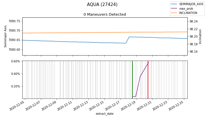 |
| Iridium 176 | Iridium 176 performed a maneuver that the maneuver detection missed. The maneuver was made inside of the SOCRATES prediction window, but the maneuver came after the probability has already dropped back to 0%. Iridium 176's maneuver was unrelated to the SOCRATES prediction. | 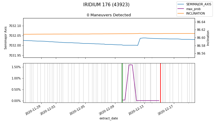 |
| Gaofen 1-04 | Gaofen 1-04 performed two maneuvers, with one of them missed by the maneuver detection. The maneuvers were made inside of the SOCRATES prediction window, but the maneuvers came after the probability has already dropped back to 0%. Gaofen 1-04's maneuver was unrelated to the SOCRATES prediction. | 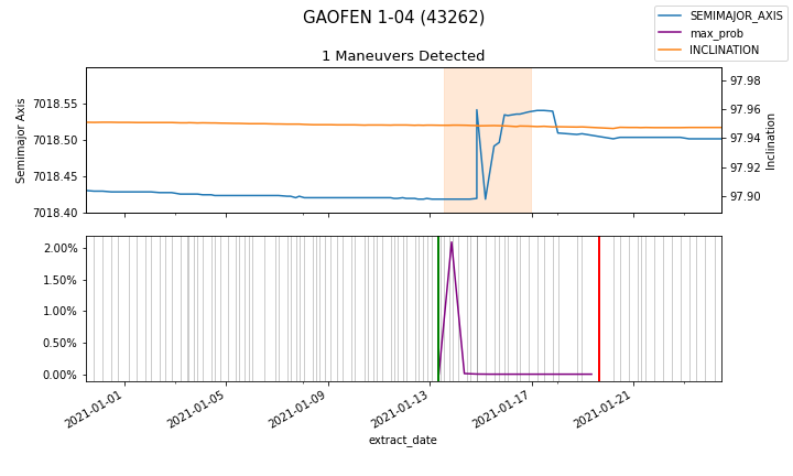 |
| Gaofen 1-02 | Gaofen 1-02 performed multiple maneuvers outside of the SOCRATES prediction window. Gaofen 1-02's maneuver was unrelated to the SOCRATES prediction. As a side note, Gaofen 1-02, Gaofen 1-03, and Gaofen 1-04 all made similar maneuvers one after another, it's unlikely that these were RMMs. | 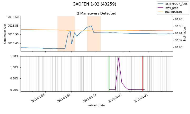 |
| Single high probability | 73 instances of the SOCRATES predictions had a single high collision chance predicted. For example, ARGOS had a very low collision chance predicted except for one instance of a 37.5% chance. | 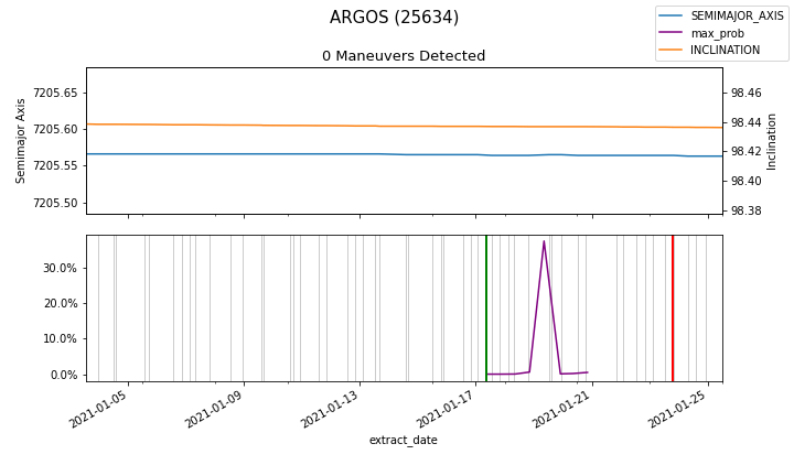 |
| Multiple high probability | 32 instances of the SOCRATES predictions had multiple high collision chance predicted. These were results that were more in line to what was expected from SOCRATES, however, no RMMs were performed for these cases. | 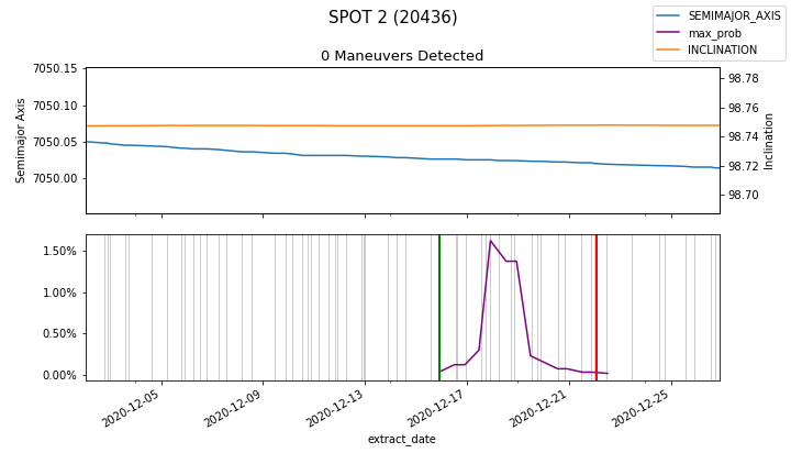 |
These results were completely unexpected, with the European Space Agency having a threshold of 0.01% collision chance to perform RMMs, seeing all 131 of these >0.5% events not having any RMMs was both shocking and surprising. It also shows that using TLEs and SGP4 trajectory calculations are very unsuitable for collision detection, even as an early warning or first pass calculations, due to their inaccuracies.
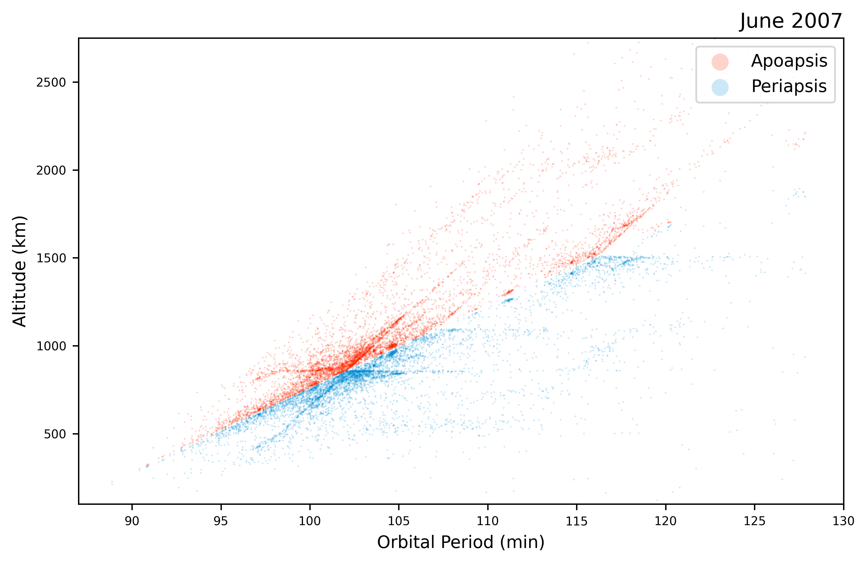
The growth of debris in LEO as well as contributions by individual debris generating events can be visualized as a Gabbard diagram animation. Each object is represented by two points in the Gabbard diagram, a lower periapsis point and a higher apoapsis along the same x-axis. An object with an elliptical orbit will have the two points further away, while a stationary orbit will have points close together. A diagonal border separating the periapsis and apoapsis points formed by circular orbits of varying orbital periods can be seen on the diagram.
Orbits decay naturally due to various factors and the points on the Gabbard diagram will appear to move towards the bottom left corner. For orbits around earth, factors such as atmospheric drag and thermal radiation can affect satellites at altitudes as high as 700–800 km during periods of increased solar activity. Higher rates of orbital decay can be observed during periods with increased solar activtiy in 1979, 1989, 2001, 2003, 2011, and 2014.
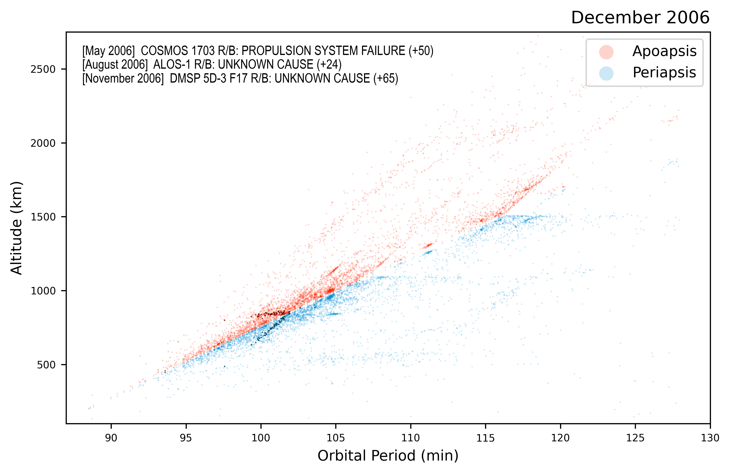
Highlighting data points with a different color and adding text annotations can add much needed context context to the visualizations. Here, text and color annotations were added to emphasize the cause and magnitude of the breakup events.
 |
 |
 |
| No annotation | Smaller Breakup Event | Huge Breakup Event |
Note: Due to small particle sizes, full screen viewing is recommended.
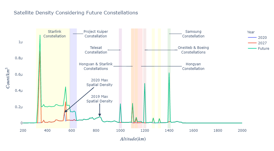
At present, there are several satellite constellations in orbit around Earth. Although, the largest without considering Starlink is Iridium NEXT with 66 satellites, Starlink has quickly taken over as the single largest satellite constellation in LEO. Knowing that current Starlink satellites are only a sliver of what SpaceX has planned, several new companies are looking to make their mark in space, increasing concerns of what this congestion will cause future space missions. Several new companies like Amazon, Samsung, and Boeing, among others, have made proposals to add thousands of satellites into Earth's orbit. The following graph models, at a very high-level, what this future spatial density could look like in LEO.
Some believe that congestion in low Earth orbit will reach a tipping point in the near future, while others believe that the issue is not imminent due to the speed at which objects decay compared to other orbits. Our analysis found support for both arguments as significant differences in satellite decay speed is observed between lower and higher orbits within LEO.
With the unprecedented launch of satellite constellations planned by SpaceX, OneWeb, Amazon, and other private companies, a multi-faceted approach will be necessary to address the potential of catastrophic events with lasting effect in LEO's higher orbits. A combination of autonomous collision avoidance systems, new international laws for decommissioning satellites, and new technologies for cleaning up defunct satellites and debris will be necessary.
We also found that meaningful conjunction prediction is no longer possible due to the increasing number of satellites and precision limitations with TLE data. In future studies, we can leverage machine learning techniques using non-public data provided by US Space Command. If our request was granted, we could more accurately analyze the impact of increasing LEO density on collision probability.
The team divided the work for this project in the following ways:
| Name | Activity |
|---|---|
| Tim Chen |
|
| Sophie Deng |
|
| Nicholas Miller |
|
gp and gp_history request classes.